https://doi.org/10.53656/nat2022-5.03

Резюме. In this paper, a deterministic model SEIR-SEI model of malaria transmission consisting of systems of ordinary differential equations, describing the transmission of malaria between humans and female anopheles mosquitoes, the definitive hosts of Plasmodium parasites, is examined. The reproduction number is estimated and the model equilibria and their stabilities are discussed. The diseasefree equilibrium for the model is found to be locally asymptotically stable if the reproduction number is less than one and unstable if the reproduction number is greater than one. Numerical simulations are carried out to demonstrate the analytical results, and suggest that malaria can be controlled by reducing the contact rate between human and mosquito, the use of active malaria drugs, insecticides and the use of mosquito treated nets.

Ключови думи: SEIR-SEI model; malaria; plasmodium; parasite; anopheles; transmission mechanism; stability, reproduction number, endemic equilibrium

Introduction

Malaria is one of the most dangerous infectious disease caused by Plasmodium parasites that are transmitted to people through the bites of infected female Anopheles mosquitoes. Malaria has claimed numerous lives around the world, about 33 billion individuals or one-half of the globes populace in 104 nations are at the threat of getting infected by malaria disease \({ }^{1)}\). It was predicted that between 300 and five hundred million individuals die of malaria yearly. Malaria is an old disease possessing a big social financial and wellness burden, it is mainly found in the tropical nations. Despite the fact that the disease was examined for centuries it still remains a primary public health concern along with 109 nations proclaimed as endemic to the disease in 2008. There were 243 million malaria cases disclosed and almost a million fatalities predominantly of little ones under 5 years without efficient vaccination in sight and most of the older antimalarial medications dropping efficiency because of the parasite advancing drug resistance, deterrence making use of bed nets is still the merely recommendations provided to infected individuals. Malaria has additionally acquired prominence in latest times since weather change or global warming is forecasted to have unanticipated impacts on its incidence each increase caused by fluctuation in temperature level influences the vector and parasite life cycle, this can easily trigger decreased occurrence of the disease in some places while it might increase in others areas.

Mathematical models for the transmission mechanics of malaria have a background of over 100 years. Mathematical models are useful in providing better understandings into the behaviour of the disease; the models have played excellent parts in affecting the decision-making process concerning treatment tactics for preventing and regulating the insurgence of malaria. Amongst all areas in biology, scientists in infectious disease were one of the primary to discover the vital function of mathematics and mathematical models in offering an specific structure for comprehending the disease transmission mechanics within and between hosts and parasites. In a mathematical model, several well-known medical and biological details are featured in a streamlined form through selecting attributes that appear to be vital to the concern being explored in disease progression and mechanics. As a result, a model is an estimation of the complex reality and its framework hinges on the methods being examined and intended for extrapolation based on the concerns being inquired. These studies can aid the fitting of empirical observations and can be applied to make theoretical forecasts on known or unidentified conditions. For instance, mathematical models have been extensively utilized by epidemiologists as tools to forecast the incident of upsurges of infectious diseases and as a resource for assisting research for eradication of malaria.

The earliest model on transmission of malaria parasite was proposed by Ross in 1911 who was awarded the nobel prize in physiology or medicine in 1902, for being the discoverer of the life cycle of malarial parasite. The Ross’s model contain two non-linear differential equations in pair of state variables that represent the proportions of infected humans and the infected mosquito. Macdonald (1957) improved Ross’s differential equations model along with some biological presumptions and entomological field data. The Ross-Macdonald model captures the vital feature of malaria transmission and the modelling structure has extensively been used to examine the epidemiology of malaria and other mosquito-borne or even vector-borne disease (Reiner et al. 2013). Jin et al. (2020) added the quarantine compartment to the Ross-Macdonald model to better study the dynamics of the transmission of malaria. Ever since the earliest model proposed by Ross, a number of models have been done for malaria by a number of authors. For instance, Aron & May (1982), Chitnis et al. (2008, 2010), Khan et al. (2015), Traore et al. (2018) included different components of malaria to the model of Macdonald featuring an incubation period in the mosquito superinfection and a duration of immunity in humans. Aron & May (1982) formed an SIRS model along with constant infection rate to fit data on age-prevalence curves. Ngwa & Shu (2000) developed a compartmental model along with an SEIRS pattern for individuals and an SEI pattern for mosquitoes, their model was extended by Chitnis et al. (2006) by means of featuring constant migration of susceptible individuals and generalizing mosquito biting rate. Although, it was presumed that individuals in the recovered class are invulnerable, in the sense that they do not experience serious disease and do not contract clinical malaria, it was argued that they still have little level of plasmodium in their blood stream and can contaminate the susceptible mosquitoes (Bai 2015; Macdonald 1957; Ngwa & Shu 2000; Traore, Singapore & Traore 2017).

Several other aspects taken into consideration in malaria models have aroused considerably interest in recent years, like the impacts of environment on the mechanics of the vector populace and the biting rate from mosquitoes to individual (Khan et al. 2015; Zhang, Jia & Song 2014; Li et al. 2002; Parham & Michael 2010), the phase framework of the duration in the hosts (Diekmann, Heesterbeek & Metz 1990; Khan et al. 2015), seasonal individual migration (Gao et al. 2014), drug resistance (Koella & Antia 2003), seasonality and spatial distribution by Plasmodium species (Zang et al. 2014) and the kind of incidence function. For instance, Traore et al. (2018) and Koutou et al. (2018a) have shown a non-autonomous model and an autonomous model for malaria transmission including the premature phases of the mosquitoes respectively. Olaniyi & Obabiyi (2013) and Koutou et al. (2018b) studies the nonlinear force of incidence of malaria between human populace and the mosquito parasites. Hasibeder & Dey (1988) and Gao et al. (2019) revealed that non-homogeneous interaction between individual and mosquitoes triggers a higher basic reproduction number using Lagragian and Eulerian techniques respectively. During the proliferation of the epidemic, time delays exist since an individual might not be infectious until some time after ending up being infected (Beretta & Kuang 2002; Zhang et al. 2014), which requires some time before the infective organism builds in the vector to the level that allows transmission of the infection to others (Khan et al. 2015; Van den Driessche & Watmough, 2002). Ruan et al. (2008) proposed a delayed Ross-Macdonald model in consideration of the incubation periods of parasites within each humans and mosquitoes. Abu-Raddad et al. (2006) and Mukandavire et al. (2009) examined the influence of the communication between HIV and malaria in an area. Variation in susceptibility exposedness and infectivity between non-immune as well as semi-immune individual hosts for malaria transmission were examined by Ducrot et al. (2009).

In this work, we examine the development of malaria, specifically; we take into consideration the interaction between individual and anopheles mosquito populace both of which are required for the life cycle of Plasmodium. Besides, we respectively examine the stability of the non-trivial disease-free equilibrium and the endemic equilibrium.

Mathematical Model and Formulation

The formulation of the model is for both human populace as well as mosquito populace at time \(t\). We divide the human populace into four classes: Susceptible \(S_{H}\), Exposed \(E_{H}\), Infectious \(I_{H}\), and Recovery Human \(R_{H}\), and that of the populace of anopheles mosquitoes is divided into three classes they are susceptible \(S_{V}\), Exposed \(E_{V}\), Infectious \(I_{V}\) respectively. The interaction between the human and anopheles mosquitoes is shown in the schematics diagram in Figure 1.

The model equation are given by:

\(\left\{\begin{array}{l}\tfrac{d S_{H}}{d t}=\gamma_{H}-b \beta_{H} S_{H} I_{V}-\mu_{H} S_{H}+w_{H} R_{H} \\ \tfrac{d E_{H}}{d t}=\beta_{H} S_{H} I_{V}-\left(\alpha_{1 H}+\mu_{H}\right) E_{H} \\ \tfrac{d I_{H}}{d t}=\alpha_{1 H} E_{H}-\left(\alpha_{2 H}+\mu_{H}+\delta\right) I_{H} \\ \tfrac{d R_{H}}{d t}=\alpha_{2 H} I_{H}-\left(\mu_{H}+w_{H}\right) R_{H} \\ \tfrac{d S_{V}}{d t}=\gamma_{V}-\beta_{V} S_{V} I_{H}-\mu_{V} S_{V} \\ \tfrac{d E_{V}}{d t}=\beta_{V} S_{V} I_{H}-\left(\alpha_{1 V}+\mu_{V}\right) E_{V} \\ \tfrac{d I_{V}}{d t}=\alpha_{1 V} E_{V}-\left(\mu_{V}+\delta_{V}\right) I_{V}\end{array}\right. \quad\quad\quad(1)\)

with the initial condition: where \(w_{H}\) is the rate lost of immunity in humans \(\delta_{V} \delta_{V}\) is the disease-induced death rate of mosquito \(S_{H}(0) \gt 0, E_{H}(0) \geq 0, I_{H}(0) \geq 0, R_{H}(0) \geq 0, S_{V}(0) \gt 0, E_{V}(0) \geq 0, I_{V}(0) \geq 0\). The term \(\beta_{H} S_{H} I_{V} \beta_{H} S_{H} I_{V}\) refers to the rate at which the human hosts get infected by the anopheles mosquitoe vector \(I_{V} I_{V}\) while the term \(\beta_{V} S_{V} I_{H} \beta_{V} S_{V} I_{H}\) refers to the rate at which the susceptible mosquitoes are infected by the human hosts \(I_{H} I_{H}\) at a time. These two tems are the primary parts of the model describing the interaction between the human host and the vector.

We also consider the following equations:

\[ N_{H}(t)=S_{H}(t)+E_{H}(t)+I_{H}(t)+R_{H}(t) \]

then the derivatives of \(N_{H}(t) N_{H}(t)\) with respect to \(t t\) is given by:

\[ \begin{gathered} \tfrac{d N_{H}}{d t} \leq \gamma_{H}-\mu_{H} N_{H}-\delta I_{H} \\ \lim _{t \rightarrow \infty} N_{H}(t) \leq \tfrac{\gamma_{H}}{\mu_{H}} \end{gathered} \]

The derivative of \(N_{V}(t) N_{V}(t)\) with respect to tt is given by:

\[ \begin{aligned} & \tfrac{d N_{V}}{d t} \leq \gamma_{V}-\mu_{V} N_{V} \\ & \lim _{t \rightarrow \infty} N_{V}(t) \leq \tfrac{\gamma_{V}}{\mu_{V}} \end{aligned} \]

It is easy to see that that has the disease-free equilibrium \(E_{0 H V}=\left(\tfrac{\gamma_{H}}{\mu_{H}}, 0,0,0, \tfrac{\gamma_{V}}{\mu_{V}}, 0,0\right)\).

Basic Reproduction Number

To compute the basic reproduction number \(R_{0} R_{0}\) for the human and mosquito of the model (1), the next-generation matrix technique is adopted.

The infection matrix is

(3)\[ F=\left(\begin{array}{cccc} 0 & \beta_{H} & 0 & \beta_{V} \\ 0 & 0 & 0 & 0 \\ 0 & 0 & 0 & 0 \\ 0 & 0 & 0 & 0 \end{array}\right) \]

The transition matrix is

(4)\[ V=\left(\begin{array}{llll} \left(\alpha_{1 H}+\mu_{H}\right) & 0 & 0 & 0 \\ -\alpha_{1 H} & \left(\alpha_{2 H}+\mu_{H}+\delta\right) & 0 & 0 \\ 0 & 0 & \left(\alpha_{1 V}+\mu_{V}\right) & 0 \\ 0 & 0 & -\alpha_{1 V} & \left(\mu_{V}+\delta_{V}\right) \end{array}\right) \]

The reproduction number for model (1) is

(5)\[ R_{1}=\rho\left(F V^{-1}\right)=\tfrac{\beta_{H}}{\alpha_{2 H}+\mu_{H}+\delta}+\tfrac{\alpha_{1 V} \beta_{V}}{\left(\alpha_{2 H}+\mu_{H}+\delta\right)\left(\mu_{V}+\delta_{V}\right)} \]

\(R_{1}=R_{0 H}+R_{0 V}\) is the spectral radius such that

\(R_{0 H}\) and \(R_{0 v} R_{0 H}\) and \(R_{0 v}\) measures the contribution from humans and Plamodium Falciparum respectively.

Stability of Disease-Free Equilibrium

Theorem 1: The disease-free equilibrium \(E_{0 H V}=\left(\tfrac{\gamma_{H}}{\mu_{H}}, 0,0,0, \tfrac{\gamma_{V}}{\mu_{V}}, 0,0\right)\) \(E_{0 H V}=\left(\tfrac{\gamma_{H}}{\mu_{H}}, 0,0,0, \tfrac{\gamma_{V}}{\mu_{V}}, 0,0\right)\) of the system of the \(O D E^{\prime} \mathrm{s}\) (1) is asymptotically stable if \(R_{1} \lt 1\) and unstable if \(R_{1} \gt 1\).

we determine the local geometric al properties of the disease-free equilibrium \(E_{0 H v}=\left(\tfrac{\gamma_{H}}{\mu_{H}}, 0,0,0, \tfrac{\gamma_{V}}{\mu_{v}}, 0,0\right) E_{0 H v}=\left(\tfrac{\gamma_{H}}{\mu_{H}}, 0,0,0, \tfrac{\gamma_{V}}{\mu_{v}}, 0,0\right)\) by considering the linearised system of ODE’s (1) by taking the Jacobian matrix and obtained. To get \(J_{0} \rightarrow S_{H}, E_{H}, I_{H}, R_{H} J_{0} \rightarrow S_{H}, E_{H}, I_{H}, R_{H}\) is been reduce to 1 in equation (1)

\(I_{H V}\left(S_{H}, E_{H}, I_{H}, R_{H}, S_{v}, E_{V}, I_{V}\right)=\left[\begin{array}{ll} \mathcal{J}_{0} & \mathcal{J}_{2} \\ \mathcal{J}_{1} & \mathcal{J}_{3} \end{array}\right] \quad \quad \quad \quad \quad(6)\)

where \[ \mathcal{J}_{0}=\left[\begin{array}{ccc} -\beta_{H} I_{H}-\mu_{H}+w_{H} R_{H} & 0 & -\beta_{H} S_{H} \\ 0 & -\left(\alpha_{1 H}+\mu_{H}\right) & \beta_{H} S_{H} \\ 0 & \alpha_{1 H} & -\left(\alpha_{2 H}+\mu_{H}+\delta\right) \end{array}\right] \] \[ \begin{aligned} \mathcal{J}_{1} & =\left[\begin{array}{lll} 0 & 0 & \alpha_{2 H} \\ 0 & 0 & 0 \\ 0 & 0 & 0 \\ 0 & 0 & 0 \end{array}\right] \\ \mathcal{J}_{2} & =\left[\begin{array}{llll} 0 & 0 & 0 & 0 \\ 0 & 0 & 0 & 0 \\ 0 & 0 & 0 & 0 \end{array}\right] \\ \mathcal{J}_{3} & =\left[\begin{array}{cccc} -\mu_{H} & 0 & 0 & 0 \\ 0 & -\beta_{V} I_{V}-\mu_{V} & 0 & -\beta_{V} S_{V} \\ 0 & 0 & -\left(\alpha_{1 V}+\mu_{V}\right) & -\beta_{V} S_{V} \\ 0 & 0 & \alpha_{1 V} & -\left(\mu_{V}+\delta_{V}\right) \end{array}\right] \end{aligned} \]

The local stability of the disease-free equilibrium determined from the Jacobian matrix (6). This implies that the Jacobian matrix of the disease-free equilibrium is given by:

\(\mathcal{J}\left(E_{0 H v}\right)=\left[\begin{array}{ll}\jmath_{0} & \jmath_{2} \\ \jmath_{1} & \jmath_{3}\end{array}\right] \quad\quad\quad\quad\quad(7)\)

\(\mathcal{J}_{0}=\left[\begin{array}{ccc}-\mu_{H} & 0 & -\beta_{H} \tfrac{\gamma_{H}}{\mu_{H}} \\ 0 & -\left(\alpha_{1 H}+\mu_{H}\right) & \beta_{H} \tfrac{\gamma_{H}}{\mu_{H}} \\ 0 & \alpha_{1 H} & -\left(\alpha_{2 H}+\mu_{H}+\delta\right),\end{array}\right]\),

\(\mathcal{J}_{1}=\left[\begin{array}{ccc}0 & 0 & \alpha_{2 H} \\ 0 & 0 & 0 \\ 0 & 0 & 0 \\ 0 & 0 & 0\end{array}\right], \quad \mathcal{J}_{2}=\left[\begin{array}{llll}0 & 0 & 0 & 0 \\ 0 & 0 & 0 & 0 \\ 0 & 0 & 0 & 0\end{array}\right]\)

and

\(\mathcal{J}_{3}=\left[\begin{array}{cccc}-\mu_{H} & 0 & 0 & 0 \\ 0 & -\mu_{V} & 0 & -\beta_{V} \tfrac{\gamma_{V}}{\mu_{V}} \\ 0 & 0 & -\left(\alpha_{1 V}+\mu_{V}\right) & -\beta_{V} \tfrac{\gamma_{V}}{\mu_{V}} \\ 0 & 0 & \alpha_{1 V} & -\left(\mu_{V}+\delta\right)\end{array}\right]\)

The determinant of (7) is given by:

\(\left|\mathcal{J}\left(E_{0 H v}\right)-\lambda I\right|=\left|\begin{array}{ll} J_{0} & J_{2} \\ J_{1} & J_{3} \end{array}\right|=0 \quad\quad\quad\quad\quad\quad(8)\)

Where:

\[ \begin{aligned} & \mathcal{J}_{0}=\left[\begin{array}{ccc} -\mu_{H}-\lambda & 0 & -\beta_{H} \tfrac{\gamma_{H}}{\mu_{H}} \\ 0 & -\left(\alpha_{1 H}+\mu_{H}\right)-\lambda & \beta_{H} \tfrac{\gamma_{H}}{\mu_{H}} \\ 0 & \alpha_{1 H} & -\left(\alpha_{2 H}+\mu_{H}+\delta\right)-\lambda \end{array}\right], \\ & \mathcal{J}_{1}=\left[\begin{array}{cccc} 0 & 0 & 0 & \alpha_{2 H} \\ 0 & 0 & 0 & 0 \\ 0 & 0 & 0 & 0 \end{array}\right], \end{aligned} \]

\[ \mathcal{J}_{2}=\left[\begin{array}{llll} 0 & 0 & 0 & 0 \\ 0 & 0 & 0 & 0 \\ 0 & 0 & 0 & 0 \end{array}\right] \]

and

\[ \mathcal{J}_{3}=\left[\begin{array}{cccc} -\mu_{H}-\lambda & 0 & 0 & 0 \\ 0 & -\mu_{V}-\lambda & 0 & -\beta_{V} \tfrac{\gamma_{V}}{\mu_{V}} \\ 0 & 0 & -\left(\alpha_{1 V}+\mu_{V}\right)-\lambda & -\beta_{V} \tfrac{\gamma_{V}}{\mu_{V}} \\ 0 & 0 & \alpha_{1 V} & -\left(\mu_{V}+\delta\right)-\lambda \end{array}\right] \]

The eigenvalues of the (8) is given by: Clearly \(\lambda=-\mu_{H}, \lambda=-\mu_{V}\) \(\lambda=-\mu_{H}, \lambda=-\mu_{V}\) are negatives and

\(\lambda^{4}+p_{1} \lambda^{3}+p_{2} \lambda^{2}+p_{3} \lambda+p_{4}=0 \quad\quad\quad\quad\quad\quad\quad\quad\quad\quad\quad(9)\)

By using the Routh-Hurwitz criterion, It can be seen that all the eigenvalues of the characteristic equation (9) have negative real part if and only if:

\(\left\{\begin{array}{l} p_{1} \gt 0, p_{2} \gt 0, p_{3} \gt 0, p_{4} \gt 0, p_{1} p_{2} p_{3}-p_{3}^{2}-p_{1}^{2} p_{4} \gt 0 \\ p_{1} p_{2} p_{3} p_{4}-p_{2} p_{3}^{2} p_{4} \gt 0 \end{array}\right. \quad\quad\quad\quad\quad\quad(10)\)

where \(p_{1}=\alpha_{1 H}+2 \mu_{H}+\alpha_{2 H}+\delta+2 \mu_{V}+\alpha_{1 V}\)

\[ \begin{aligned} & p_{2}=2 \alpha_{1 H} \mu_{V}+4 \mu_{V} \mu_{H}+2 \alpha_{2 H} \mu_{V}+\alpha_{1 H} \alpha_{1 V}+\alpha_{2 H} \alpha_{1 V}+\delta \alpha_{1 V}+2 \alpha_{1 V} \mu_{H}+\alpha_{1 V} \mu_{V}^{3} \\ & \quad-\tfrac{\alpha_{1 V} \beta_{V} \gamma_{V}}{\mu_{V}}-\tfrac{\beta_{H} \gamma_{H}}{\mu_{H}} \\ & p_{3}=\alpha_{1 H} \alpha_{2 H}+\alpha_{1 H} \mu_{H}+\alpha_{1 H} \delta+\alpha_{2 H} \mu_{H}+\mu_{H}^{2}+\delta \mu_{H}+2 \alpha_{1 H} \alpha_{2 H} \mu_{V}+2 \alpha_{1 H} \mu_{V} \mu_{H} \\ &+2 \alpha_{1 H} \delta \mu_{V}+2 \alpha_{1 H} \mu_{V} \mu_{H}+2 \mu_{V} \mu_{H}^{2}+\alpha_{1 H} \alpha_{2 H} \alpha_{1 V}+\alpha_{1 H} \alpha_{1 V} \mu_{H}+\alpha_{1 H} \alpha_{1 V} \mu_{H} \\ &+\alpha_{2 H} \alpha_{1 V} \mu_{H}+\alpha_{1 V} \mu_{H}^{2}+\alpha_{1 H} \alpha_{1 V} \delta \mu_{V}^{3}+2 \alpha_{1 V} \delta \mu_{V}{ }^{3} \mu_{H}+\alpha_{1 V}{ }^{3} \mu_{V}^{3} \\ &+\alpha_{1 V} \delta_{V}^{3}-\tfrac{\alpha_{1 H} \alpha_{1 V} \beta_{V} \gamma_{V}}{\mu_{V}}-\tfrac{2 \alpha_{1 V} \mu_{H} \beta_{V} \gamma_{V}}{\mu_{V}}-\tfrac{\alpha_{1 V}^{2} \beta_{V} \gamma_{V}}{\mu_{V}}-\tfrac{\alpha_{1 V} \delta \beta_{V} \gamma_{V}}{\mu_{V}} \\ &-\tfrac{2 \mu_{V} \beta_{H} \gamma_{H}}{\mu_{H}}-\tfrac{\alpha_{1 V} \beta_{H} \gamma_{H}}{\mu_{H}} \\ & p_{4}=\alpha_{1 H} \alpha_{2 H} \alpha_{1 V} \mu_{V}{ }^{3}+\alpha_{1 H} \alpha_{1 V} \mu_{V}{ }^{3} \mu_{H}+\alpha_{1 H} \alpha_{1 V} \delta \mu_{V}{ }^{3}+\alpha_{2 H} \alpha_{1 V} \mu_{V}{ }^{3} \mu_{H}+\alpha_{1 V} \mu_{V}{ }^{3} \mu_{H}^{2} \\ &+\delta \alpha_{1 V} \mu_{V}{ }^{3} \mu_{H}+\tfrac{\alpha_{1 V} \beta_{V} \gamma_{V} \beta_{H} \gamma_{H}}{\mu_{V} \mu_{H}}-\tfrac{\alpha_{1 V} \beta_{H} \gamma_{H} \mu_{V}}{\mu_{H}}-\tfrac{\beta_{H} \gamma_{H} \mu_{V}^{2}}{\mu_{H}} \\ &-\tfrac{\alpha_{1 H} \alpha_{2 H} \alpha_{1 V} \beta_{V} \gamma_{V}}{\mu_{V}}-\tfrac{\alpha_{1 H} \mu_{H} \beta_{V} \gamma_{V}}{\mu_{V}}-\tfrac{\alpha_{1 H} \alpha_{1 V} \delta \beta_{V} \gamma_{V}}{\mu_{V}}-\tfrac{\alpha_{2 H} \alpha_{1 V} \mu_{H} \beta_{V} \gamma_{V}}{\mu_{V}} \\ &-\tfrac{\alpha_{1 V} \mu_{V}^{2} \beta_{V} \gamma_{V}}{\mu_{V}}-\tfrac{\delta \alpha_{1 V} \mu_{H} \beta_{V} \gamma_{V}}{\mu_{V}} \end{aligned} \]

It can be seen that all the eigenvalues have negative real parts and therefore the disease free equilibrium is Locally asymptotically stable.

Endemic Equilibrium

We consider a situation in which all the steady states coexist in the equilibrium. We denote \(E_{H V}^{*}=\left(S_{H}{ }^{*}, E_{H}{ }^{*}, I_{H}{ }^{*}, R_{H}{ }^{*}, S_{V}{ }^{*}, E_{V}{ }^{*}, I_{V}{ }^{*}\right)\) \(E_{H V}^{*}=\left(S_{H}{ }^{*}, E_{H}{ }^{*}, I_{H}{ }^{*}, R_{H}{ }^{*}, S_{V}{ }^{*}, E_{V}{ }^{*}, I_{V}{ }^{*}\right)\) as the endemic equilibrium of the system (1) we also obtain

\[ S_{H}^{*}=\tfrac{\left(\alpha_{1 H}+\mu_{H}\right)-\left(\alpha_{2 H}+\mu_{H}+\delta\right)}{\alpha_{1 H} \beta_{H}} \]

\[ \begin{aligned} E_{H}^{*} & =\tfrac{\alpha_{1 H} \beta_{H} \gamma_{H}-\mu_{H}\left(\alpha_{1 H}+\mu_{H}\right)\left(\alpha_{2 H}+\mu_{H}+\delta\right)}{\alpha_{1 H} \mu_{H} \beta_{H}\left(\alpha_{1 H}+\mu_{H}\right)} \\ I_{H}^{*} & =\tfrac{\alpha_{1 H} \beta_{H} \gamma_{H}-\mu_{H}\left(\alpha_{1 H}+\mu_{H}\right)\left(\alpha_{2 H}+\mu_{H}+\delta\right)}{\beta_{H}\left(\alpha_{2 H}+\mu_{H}+\delta\right)\left(\alpha_{1 H}+\mu_{H}+w_{H}\right)} \\ R_{H}^{*} & =\tfrac{\alpha_{2 H}\left(\alpha_{1 H} \beta_{H} \gamma_{H}-\mu_{H}\right)\left(\alpha_{1 H}+\mu_{H}\right)\left(\alpha_{2 H}+\mu_{H}+\delta_{H}\right)}{\beta_{H}\left(\alpha_{2 H}+\mu_{H}+\delta\right)\left(\mu_{H}+w_{H}+\alpha_{1 H}\right)} \\ E_{V}^{*} & =\tfrac{\alpha_{1 V} \beta_{V} \gamma_{V}-\mu_{V}^{2}\left(\alpha_{1 V}+\mu_{V}\right)\left(\mu_{V}+\delta_{V}\right)}{\alpha_{1 V} \beta_{V}\left(\alpha_{1 V}+\mu_{V}\right)} \\ I_{V}^{*} & =\tfrac{\alpha_{1 V} \beta_{V} \gamma_{V}-\mu_{V}^{2}\left(\alpha_{1 V}+\mu_{V}\right)\left(\mu_{V}+\delta_{V}\right)}{\alpha_{1 V} \beta_{V}\left(\alpha_{1 V}+\mu_{V}\right)} \end{aligned} \]

To find \(S_{V}^{*} S_{V}^{*}\). We find the determinant of the matrix \(\mathcal{J}_{3}\)

\[ \begin{aligned} & \left(\alpha_{1 V}+\mu_{V}\right)\left(\mu_{V}+\delta_{V}\right)-\alpha_{1 V} \beta_{V} S_{V}^{*} \\ & \tfrac{\left.\left(\alpha_{1 V}\right)+\mu_{V}\right)\left(\mu_{V}+\delta_{V}\right)}{\alpha_{1 V} \beta_{V}}=S_{V}^{*} \\ & S_{V}^{*}=\tfrac{\left(\alpha_{1 V}+\mu_{V}\right)\left(\mu_{V}+\delta_{V}\right)}{\alpha_{1 V} \beta_{V}} \end{aligned} \]

The local stability of the endemic equilibrium determined from the Jacobian Matrix (6). This implies that the Jacobian matrix of the endemic equilibrium is given by: \(\mathcal{J}\left(S_{H}{ }^{*}, E_{H}{ }^{*}, I_{H}{ }^{*}, R_{H}{ }^{*}, S_{V}{ }^{*}, E_{V}{ }^{*}, I_{V}{ }^{*}\right) \mathcal{J}\left(E^{*}{ }_{H V}\right)=\left[\begin{array}{ll}J_{0} & J_{2} \\ J_{1} & J_{3}\end{array}\right]\)

Where:

\[ \mathcal{J}_{0}=\left[\begin{array}{ccc} -\beta_{H} I_{H}^{*}-\mu_{H}+w_{H} R_{H} & 0 & -\beta_{H} S_{H}^{*} \\ 0 & -\left(\alpha_{1 H}+\mu_{H}\right) & \beta_{H} S_{H}^{*} \\ 0 & \alpha_{1 H} & -\left(\alpha_{2 H}+\mu_{H}+\delta\right) \end{array}\right] \]

\[ \begin{aligned} \mathcal{J}_{1} & =\left[\begin{array}{ccc} 0 & 0 & \alpha_{2 H} \\ 0 & 0 & 0 \\ 0 & 0 & 0 \\ 0 & 0 & 0 \end{array}\right] \\ \mathcal{J}_{2} & =\left[\begin{array}{llll} 0 & 0 & 0 & 0 \\ 0 & 0 & 0 & 0 \\ 0 & 0 & 0 & 0 \end{array}\right] \end{aligned} \]

and

\[ \mathcal{J}_{3}=\left[\begin{array}{cccc} -\mu_{H} & 0 & 0 & 0 \\ 0 & -\beta_{v} I_{v}-\mu_{V} & 0 & -\beta_{V} S_{V}^{*} \\ 0 & 0 & -\left(\alpha_{1 V} \mu_{V}\right) & \beta_{V} S_{V}^{*} \\ 0 & 0 & \alpha_{1 V} & -\left(\mu_{V}+\delta_{v}\right) \end{array}\right] \]

To get \(S_{H}{ }^{*}\). We find the determinant of \(\mathcal{J}_{0}\).

\(\begin{aligned} & b=\left(\alpha_{1 H}+\mu_{H}\right)-\left(\alpha_{2 H}+\mu_{H}+\delta\right)-\alpha_{1 H} \beta_{H} S_{H}^{*}\left(\alpha_{1 H}+\mu_{H}\right)-\left(\alpha_{2 H}+\mu_{H}+\delta\right) \\ & \quad=\alpha_{1 H} \beta_{H} S_{H}^{*} \end{aligned}\quad\quad(13)\)

Divide through by \(\alpha_{1 H} \beta_{H}\)

The eigenvalues of the (13) are given by:

\(\lambda_{1}=-\left[\tfrac{\left(\alpha_{1 H}+\mu_{H}\right)\left(\alpha_{2 H}+\mu_{H}+\delta\right)}{\alpha_{1 H}}+\mu_{H}\right], \quad \lambda_{2}=-\mu_{H}\), \(\lambda_{3}=-\tfrac{\alpha_{1 V} \beta_{V} \gamma_{V}}{\mu_{V}\left(\alpha_{1 V}+\mu_{V}\right)\left(\mu_{V}+\delta_{V}\right)}\)

Which are negatives and

(14)\(\lambda^{4}+q_{1} \lambda^{3}+q_{2} \lambda^{2}+q_{3} \lambda+q_{4}=0\)

By Using the Routh-Hurwitz criterion, it can be seen that all the eigenvalues of the characteristic equation (14) have negative real part if and only if:

(15)\(\left\{\begin{array}{c}q_{1} \gt 0, q_{2} \gt 0, q_{3} \gt 0, q_{4} \gt 0, \\ q_{1} q_{2}-q_{3} \gt 0, \\ q_{1} q_{2} q_{3}-q_{3}^{2}-q_{1}^{2} q_{4} \gt 0 \\ q_{1} q_{2} q_{3} q_{4}-q_{2} q_{3}^{2} q_{4} \gt 0\end{array}\right.\)

Where:

\[ \begin{aligned} & q_{2}=\alpha_{1 H} \alpha_{2 H}+4 \alpha_{1 H} \mu_{H}+2 \delta \alpha_{1 H}+\alpha_{1 H} \mu_{V}+2 \alpha_{2 H} \mu_{H}+4 \mu_{H}^{2}+\delta_{H}+2 \mu_{H} \mu_{V} \\ &+2 \mu_{H} \alpha_{1 V}+\alpha_{2 H} \mu_{V}+\alpha_{2 H} \alpha_{1 V}+\alpha_{2 H} \mu_{H}+\delta_{V}+\delta \alpha_{1 V}+\delta \mu_{H}+\mu_{V} \alpha_{1 V} \\ &+\mu_{V} \alpha_{1 V}+\mu_{V} \mu_{H}+\beta_{V} \alpha_{1 V}+\beta_{V} \mu_{V} \\ & q_{3}=\alpha_{1 H} \alpha_{2 H} \mu_{V}+\alpha_{1 H} \alpha_{2 H} \alpha_{1 V}+\alpha_{1 H} \alpha_{2 H} \mu_{H}+\alpha_{1 H} \mu_{H} \mu_{V}+\alpha_{1 H} \alpha_{2 H} \alpha_{1 V}+\alpha_{1 H} \mu_{H}^{2} \\ &+\delta \alpha_{1 H} \mu_{V}+\delta \alpha_{1 H} \alpha_{1 V}+\delta \alpha_{1 H} \mu_{V}+\alpha_{1 H} \mu_{V} \mu_{H}+\alpha_{1 H} \mu_{V} \mu_{H} \\ &+\alpha_{1 H} \beta_{V} \alpha_{1 V}+\alpha_{1 H} \beta_{V} \mu_{V}+\alpha_{2 H} \mu_{V} \mu_{H}+\mu_{H} \alpha_{2 H} \alpha_{1 V}+\mu_{H}^{2} \alpha_{2 H}+\mu_{H}^{2} \mu_{V} \\ &+\mu_{H}^{2} \alpha_{1 V}+\mu_{H}^{3}+\delta \mu_{H} \mu_{V}+\delta \mu_{H} \alpha_{1 V}+\delta \mu_{H}^{2}+2 \mu_{H}^{2} \mu_{V}+2 \alpha_{1 V} \mu_{V} \mu_{H} \\ &+\alpha_{2 H} \mu_{V} \mu_{H}+\alpha_{2 H} \beta_{V} \alpha_{1 V}+\alpha_{2 H} \beta_{V} \mu_{V}+2 \mu_{H} \beta_{V} \alpha_{1 V}+2 \mu_{H} \beta_{V} \mu_{V} \\ &+\delta \mu_{V} \mu_{H}+\delta \beta_{V} \alpha_{1 V}+\delta \beta_{V} \mu_{V}+\alpha_{1 H} \alpha_{2 H} \mu_{V}+\alpha_{1 H} \alpha_{2 H} \mu_{H}+\alpha_{1 H} \mu_{H} \mu_{V} \\ &+\alpha_{1 H} \mu_{H} \alpha_{1 V}+\alpha_{1 H} \mu_{H}^{2}+\delta \alpha_{1 H} \delta_{1 V}+\delta \alpha_{1 H} \mu_{H}+\alpha_{H} \alpha_{2 H} \mu_{V}+\alpha_{H} \alpha_{2 H} \mu_{V} \\ &+\mu_{H} \alpha_{2 H} \alpha_{1 V}+\mu_{H}^{2} \alpha_{2 H}+\mu_{H 2} \mu_{V}+\mu_{H}^{2} \alpha_{1 V}+\mu_{H}^{3}+\delta \mu_{H} \mu_{V}+\delta \alpha_{V} \mu_{H} \\ &+\delta \mu_{H}^{2}+\delta \mu_{H} \\ & q_{4}=2 \alpha_{1 H} \alpha_{2 H} \alpha_{1 V} \mu_{V}+2 \alpha_{1 H} \alpha_{2 H} \mu_{V} \mu_{H}+\alpha_{1 H} \alpha_{2 H} \mu_{V} \beta_{V}+\alpha_{1 H} \alpha_{1 V} \mu_{V} \mu_{H}+\alpha_{1 H} \mu_{H}^{2} \mu_{V} \\ &+\alpha_{1 H} \mu_{H} \beta_{V} \alpha_{1 V}+\alpha_{1 H} \mu_{H} \beta_{V} \mu_{V}+\delta \alpha_{1 H} \mu_{V} \alpha_{1 V}+\delta \alpha_{1 H} \mu_{V} \mu_{H} \\ &+\delta \alpha_{1 H} \beta_{V} \alpha_{1 V}+\delta \alpha_{1 H} \beta_{V} \mu_{V}+\alpha_{2 H} \mu_{H} \mu_{V} \alpha_{1 V}+\alpha_{2 H} \mu_{H}^{2} \mu_{V} \\ &+\alpha_{2 H} \mu_{H} \beta_{V} \alpha_{1 V}+\alpha_{2 H} \mu_{H} \beta_{V} \mu_{V}+\mu_{H}^{2} \mu_{V} \alpha_{1 V}+\mu_{H}^{3} \mu_{V}+\mu_{H}^{2} \beta_{V} \alpha_{1 V} \\ &+\mu_{H}^{2} \beta_{V} \mu_{V}+\delta \mu_{H} \mu_{V} \alpha_{1 V}+\delta \mu_{H}^{2} \mu_{V}+\delta \mu_{H} \beta_{V} \alpha_{1 V}+\delta \mu_{H} \mu_{V} \beta_{V} \\ &+\alpha_{1 H} \alpha_{2 H} \alpha_{1 V} \beta_{V}+\alpha_{1 H} \alpha_{2 H} \beta_{V} \mu_{V}+\alpha_{1 H} \mu_{H} \alpha_{1 V} \mu_{V} \\ &+\alpha_{1 H} \mu_{H}^{2} \mu_{V} \alpha_{1 H} \mu_{H} \alpha_{1 V} \beta_{V}+\alpha_{1 H} \mu_{H} \beta_{V} \mu_{V}+\delta \alpha_{1 H} \alpha_{1 V} \mu_{V}+\delta \alpha_{1 H} \\ &+\delta \alpha_{1 H} \beta_{V} \mu_{V}+\mu_{H} \alpha_{2 H} \mu_{V}+\mu_{H}^{2} \alpha_{1 V} \mu_{V}+\mu_{H} \alpha_{2 H} \beta_{V} \alpha_{1 V}+\mu_{H} \alpha_{2 H} \beta_{V} \mu_{V} \\ &+\mu_{H}^{3} \mu_{V}+\mu_{H}^{2} \beta_{V} \mu_{V}+\delta \mu_{H} \mu_{V} \alpha_{1 V}+\delta \mu_{H}^{2} \mu_{V}+\delta \mu_{H} \beta_{V} \alpha_{1 V}+\delta \mu_{H} \beta_{V} \\ &+\delta \mu_{H} \beta_{V} \mu_{V} . \end{aligned} \] Results and Discussion

The behaviour of the model using some parameter values from Olaniyi & Obabiyi (2013) as presented in Table 1 are used for simulation with the following initial conditions:

\(S_{H}(0)=100, E_{H}(0)=20, I_{H}(0)=10, R_{H}(0)=0, S_{V}(0)=1000, E_{V}(0)=20, I_{V}(0)=30\).

The numerical simulation was analysed and plotted using MATLAB and the results are shown in Figure 2 –10 to illustrate the behaviour for different values of the model parameters.

Figure 2 shows the number of individuals that are susceptible to the virus, exposed to the virus, infected with the virus and recovered from the virus (malaria). It is observed that in the human populace, the number of individual reduced drastically, while those exposed increased initially more than the infected and was later stabilized by the rate of recovery experience in the recovery class.

Figure 3 shows the number of anopheles mosquitoes that are susceptible, exposed and infected in the mosquito populace. It is observed that in the mosquito populace, the number of mosquito in susceptible class reduces, while those in the exposed class and infected class in the mosquito populace also reduces with time since there is no recovered mosquito.

Figures 4, 5, 6, 7 show the different effect of the biting rate of the mosquito on human populace. In particular, Figure 4 shows the susceptible human populace dropped as a result of the increase in infection by infectious mosquito and later stabilize by the rate of recovery. Figure 5 and Figure 6 respectively show the magnitude at which the exposed and infectious human populace experience decrease in human populace in their respective compartment as a result of increase in infection by the infectious mosquito. It is also observed that decreased in the magnitude of infection by the infectious mosquito contributes to the increase in recovered human populace as shown in Figure 7, which sequentially effected the sharp reduction experienced by susceptible human populace.

Similarly, Figure 8, Figure 9 and Figure 10 show the different effect of the biting rate by the mosquito on mosquito populace. It is observed from Figure 8 that the number of susceptible reduced with time as there are no recovered compartment for mosquito populace. However, the increase in infection rate by the mosquito populace reduces the susceptible mosquito populace as seen in Figure 8. The increase in biting rate of the infectious mosquito increases exposed anopheles mosquitoes and infectious anopheles mosquitoes as shown in Figure 9 and Figure 10 respectively. However, it should be noted if the biting rate of the mosquito can reduce, it would reduced the number of anopheles mosquitoes that would be exposed and infected and in turn will reduce the number of individuals that would be exposed and infected with malaria.

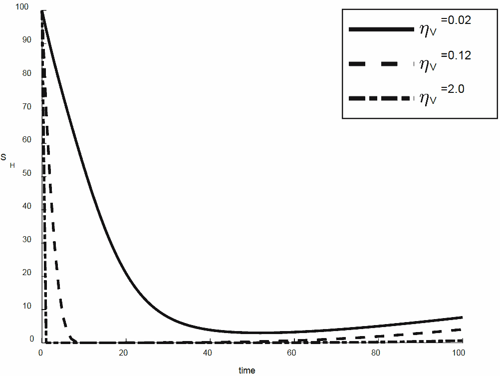
Figure 4. The behaviour of susceptible human for different values of \(\eta_{V}\)

Summary and Conclusion

Mathematical model is a useful technique for solving real life problems, a deterministic model SEIR-SEI consisting of systems of ordinary differential equations was considered in this paper. The model describes the transmission of malaria among humans populace and mosquito populace. The existence of the region where the model is epidemiologically feasible was established. The model is asymptotically stable when the reproduction number \(R_{0} \lt 1\), which implies that malaria will eventually be eliminated from the populace. But, unstable when \(R_{0} \gt 1\), which implies that malaria would continue to be prevalent among humans. Numerical simulations were conducted to further study the interaction between human populace and mosquito populace.

From the numerical results, the study concludes that increase in infection rate would cause a high increase in the number of anopheles mosquitoes that would be exposed and hereby infected causing human populace to go into extinction. To have a stable human populace, the recovery rate should be increase and infection rate between human populace and Anopheles mosquito populace should be reduced.

Accordingly, in line with the above conclusion, the following recommendation are made to keep the human populace stable: Use of mathematical models to model real life problems which simplifies problems in the society should be encouraged; Transmission of malaria can be reduced by reducing the infection rate. The method of reduction include fighting against the development of eggs, larvae and pupa by using larvicide or by cleaning the environment to reduce the breeding sites of eggs and larvae; Use of bed nets (mosquito protected nets) and insecticides to reduce contact rate between anopheles mosquitoes and humans.

NOTES

1. World Health Organization 2019. World malaria report 2019. https://www.who. int/publications-detail/world-malaria-report-2019. Accessed 08 August 2022.

REFERENCES

ABU-RADDAD, L. J., et al., 2006. Dual Infection with HIV and Malaria Fuels the Spread of Both Diseases in Sub-Saharan Africa. Science. 314, 1603 – 1606.

ARON, J. L., & MAY, R. M., 1982. The population dynamics of malaria. In: Anderson, R.M. (ed.) The Population Dynamics of Infectious Disease: Theory and Applications, Chapman & Hall, London, 139 – 179.

BAI, Z., 2015. Threshold dynamics of a periodic SIR model with delay in an infected compartment. Mathematical Biosciences and Engineering. 12(3), 555 – 564.

BERETTA, E. & KUANG, Y., 2002. Geometric Stability Switch Criteria in Delay Differential Systems with Delay Dependent Parameters. SIAM Journal on Mathematical Analysis. 33, 1144 – 1165.

CHITNIS, N. et al., 2006. Bifurcation analysis of a mathematical model for malaria transmission. SIAM Journal on Applied Mathematics. 67, 24 – 45.

CHITNIS, N. et al., 2008. Determining important parameters in the spread of malaria through the sensitivity analysis of a mathematical model. Bulletin of Mathematical Biology. 70, 1272 – 1296.

CHITNIS, N. et al., 2010. Comparing the effectiveness of malaria vector-control interventions through a mathematical model. The American Journal of Tropical Medicine and Hygiene. 83, 230 – 240.

DIEKMANN, O., HEESTERBEEK, J. A. P., & METZ, J. A. J. 1990. On the definition and the computation of the basic reproduction ratio R0 in models for infectious diseases in heterogeneous populations. Journal of Mathematical Biology. 28,365 – 382.

DUCROT, A., et al., 2009. A mathematical model for malaria involving diferential susceptibility, exposedness and infectivity of human host. Journal of Biological Dynamics. 3(6), 574 – 598.

GAO, D. et al., 2014. Optimal seasonal timing of oral azithromycin for malaria. American Journal of Tropical Medicine and Hygiene. 91(5), 936 – 942.

GAO, D. et al., 2019. Habitat fragmentation promotes malaria persistence. Journal of Mathematical Biology. 79(6 – 7), 2255 – 2280.

HASIBEDER, G. & DYE, C., 1988. Population dynamics of mosquito-borne disease: persistence in a completely heterogeneous environment. Theoretical Population Biology. 33, 31 – 53.

JIN, X., et al., 2020. Mathematical Analysis of the Ross-Macdonald Model with Quarantine. Bulletin of Mathematical Biology. 82(4):47.

KHAN, M. A. et al., 2015. Dynamical system of a SEIQV epidemic model with nonlinear generalized incidence rate arising in biology. International Journal of Biomathematics. 10(7), 1750096 (19 pages).

KOELLA J. C., & ANTIA R., 2003. Epidemiological models for the spread of antimalarial resistance. Malaria Journal, 2(3). https://doi.org/10.1186/1475-2875-2-3.

KOUTOU, O., TRAORÉ, B., & SANGARÉ, B., 2018a. Mathematical modeling of malaria transmission global dynamics: Taking into account the immature stages of the vectors. Advances in Difference Equations, 220. https://doi.org/10.1186/ s13662-018-1671-2.

KOUTOU, O., TRAORÉ B. & SANGARÉ B., 2018b. Mathematical model of malaria transmission dynamics with distributed delay and a wide class of nonlinear incidence rates. Cogent Mathematics and Statistics, 5:1. https://doi.org/10.1080/1 7513758.2018.1468935.

LI, J., et al., 2002. Dynamic Malaria Models with Environmental Changes. Proceedings of the Thirty- Fourth Southeastern Symposium on System Theory Huntsville, AL, London. 396 – 400. doi: 10.1109/ SSST.2002.1027075.

MACDONALD, G., 1957. The epidemiology and control of malaria. Oxford University Press.

MUKANDAVIRE, Z. et al., 2009. Modelling Effects of Public Health Sensitizational Campaigns on HIV-AIDS Transmission Dynamics. Applied Mathematical Modelling, 33, 2084 – 2095.

NGWA, G. A., & SHU, W. S., 2000. A mathematical model for endemic malaria with variable human and mosquito populations. Math. Comput. Model. 32, 747 – 763.

OLANIYI, S., & OBABIYI, O. S., 2013. Mathematical model for malaria transmission dynamics on human and mosquito population with non-linear forces of infectious disease. Int. Journal of Pure and Applied Mathematics. 88(1), 125 – 150.

PARHAM, P. E. & MICHAEL, E., 2010. Modeling the effects of weather and climate change on malaria transmission. Environ Health Perspect, 118, 620 – 626.

REINER, R. C., et al., 2013. A systematic review of mathematical models of mosquitoborne pathogen transmission: 1970-2010. Journal of the Royal Society Interface, 10(81), \(1-13\). https://doi.org/10.1098/rsif.2012.0921.

ROSS, R., 1911. The Prevention of Malaria. Murray, London. p. 3, 31, 48.

RUAN, S., et al., 2008. On the Delayed Ross–Macdonald Model for Malaria Transmission. Bulletin of Mathematical Biology. 70, 1098 – 1114.

TRAORÉ, B., et al., 2018. A mathematical model of malaria transmission in a periodic environment. J. Biol. Dyn. 12(1), 400 – 432.

TRAORÉ, B., SANGARÉ, B., & TRAORÉ, S., 2017. Mathematical model of malaria transmission with structured vector population and seasonality. J. Appl. Math., Article ID ID6754097. https://doi.org/10.1155/2017/6754097.

VAN DEN DRIESSCHE, P. & WATMOUGH, J., 2002. Reproduction numbers and sub-threshold endemic equilibria for compartmental models of disease transmission. Mathematical Biosciences, 180, 29 – 48.

ZHANG, Q. et al., 2014. The epidemiology of Plasmodium vivax and Plasmodium falciparum malaria in China, 2004-2012: from intensified control to elimination. Malaria Journal. 13:419. https://doi.org/10.1186/1475-2875-13-419.

ZHANG, J., JIA, J. AND SONG, X. 2014. Analysis of an SEIR Model with Saturated Incidence and Saturated Treatment Function. The Scientific World Journal. Article ID: 910421, 11 p. https://doi.org/10.1155/2014/910421.